PyG网络 (一) 图注意力神经网络GAT

下载并引入库

# Install required packages.
!pip install -q torch-scatter -f https://data.pyg.org/whl/torch-1.10.0+cu113.html
!pip install -q torch-sparse -f https://data.pyg.org/whl/torch-1.10.0+cu113.html
!pip install -q git+https://github.com/pyg-team/pytorch_geometric.git

import numpy as np
import torch
import torch.nn as nn
import torch.nn.functional as F 

消息传递网络 (Message Passing Network)

消息传递网络可以被描述为:

\[x_i^{(k)} = \gamma^{(k)} (x_i^{(k-1)}, \square_{j \in \mathcal{N}(i)} \phi^{(k)} (x_i^{(k-1)}, x_j^{(k-1)}, e_{j, i}))\]

其中 $\square$ 代表一个 可微分的 (differentiable), 且 置换不变的 (permutation invariant) 函数, 例如求和 (sum), 平均 (mean), 求最大值 (max) 等等. 而 $\gamma$ 和 $\phi$ 代表其他可微分的函数, 例如多层感知机 (Multilayer Perceptron, MLP).

具体到代码中, $\gamma$ 是 update() 函数, $\square$ 是 aggregate() 函数, $\phi$ 是 message() 函数.

让我们使用 GCNConv 来构建一个简单的图卷积层网络, 其结构如下:

from torch_geometric.nn import MessagePassing

class GCNConv(MessagePassing):
    def __init__(self, in_channels, out_channels):
        # Initialize the class, call "super" specifying your aggregations
        super(GCNConv, self).__init__(aggr='add')

    def forward(self, x, edge_index):
        # Forward and propagate
        return self.propagate(edge_index, x=x, norm=norm)

    def message(self):
        # Compute the message
        NotImplementedError

数学表达式为: $x_i^{(k)} = \sum_{j \in \mathcal{N}(i) \cup \{i\}} \frac{1}{\sqrt{\text{deg}(i)} \cdot \sqrt{\text{deg}(j)}} \cdot \bigg( \Theta \cdot x_j^{(k-1)} \bigg)$

这里我们可以使用 $\sum_{j \in \mathcal{N}(i) \cup {i}} \frac{1}{\sqrt{\text{deg}(i)} \cdot \sqrt{\text{deg}(j)}}$ 作为 $\square_{j \in \mathcal{N}(i)}$ 的具体形式, 而 $\Theta$ 为消息函数 $\phi$.

则我们构建GCN的步骤为:

添加自循环 (self-loops), 也就是使得图 $\mathcal{G}$ 内存在边 $(v, v)$.
线性变换 (linear transform) 到节点特征矩阵 (node feature matrix)
计算归一化系数
归一化节点特征
对所有邻居节点特征求和

其中, 步骤 1-3 在 forward 方法内实现, 步骤 4 在 message 方法内实现, 步骤 5 在 __init__ 内实现:

from torch_geometric.nn import MessagePassing
from torch_geometric.utils import add_self_loops, degree

class GCNConv(MessagePassing):
    def __init__(self, in_channels, out_channels):
        super(GCNConv, self).__init__(aggr='add') # Sum aggregation (step 5).
        self.linear = torch.nn.Linear(in_channels, out_channels)

    def forward(self, x, edge_index):
        # x has shape [N, in_channels]
        # edge_index has shape [2, E]

        # step 1: Add self-loops to the adjacency matrix.
        edge_index, _ = add_self_loops(edge_index, num_nodes=x.size(0))

        # step 2: Linearly transform node feature matrix.
        x = self.linear(x)

        # step 3: Compute normalization.
        row, col = edge_index
        deg = degree(col, x.size(0), dtype=x.dtype)
        deg_inv_sqrt = deg.pow(-0.5)
        norm = deg_inv_sqrt[row] * deg_inv_sqrt[col]

        # step 4-5: Start propagating messages.
        return self.propagate(edge_index, x=x, norm=norm)

    def message(self, x_j, norm):
        # x_j has shape [E, out_channels]

        # Step 4: Normalize node features
        return norm.view(-1, 1) * x_j

GAT 网络结构

同理, GAT 的网络结构也相似 [1]:

class GATLayer(nn.Module):
    """Simple PyTorch Implementation of the Graph Attention Layer."""

    def __init__(self):
        super(GATLayer, self).__init__()

    def forward(self, input, adj):
        print("") 

线性变换 (Linear Transformation)

对于单个节点的节点特征我们有:

\[\bar{h^\prime}_i = \textbf{W} \cdot \bar{h_i}\]

其中我们的输入 $\bar{h}_i \in \mathbb{R}^F$, $\textbf{W} \in \mathbb{R}^{F^\prime \times F}$. 因此我们的输出 \bar{h^\prime}_i \in \mathbb{R}^{F^\prime}. 这样我们将输入维度空间线性映射到了输出维度空间. 让我们验证一下:

in_features = 5
out_features = 2
nb_nodes = 3
np.random.seed(42)

W = nn.Parameter(torch.zeros(size=(in_features, out_features)))
# xavier paramiter inizializator
nn.init.xavier_uniform_(W.data, gain=1.414)
print('weight matrix:\n', W)

input = torch.rand(nb_nodes, in_features)
print('\ninput:\n', input)

# 线性变换
h = torch.mm(input, W)
print('\nfeature matrix:\n', h)

输出结果:

weight matrix:
 Parameter containing:
tensor([[ 0.5556, -0.5351],
        [ 0.8731,  0.0384],
        [ 0.3814,  0.0958],
        [-0.3068,  0.3968],
        [-1.1768, -0.0319]], requires_grad=True)

input:
 tensor([[0.6442, 0.5693, 0.7771, 0.0850, 0.4446],
        [0.1844, 0.7672, 0.0953, 0.0745, 0.5096],
        [0.5041, 0.6732, 0.2061, 0.1773, 0.3532]])

feature matrix:
 tensor([[ 0.6022, -0.2289],
        [ 0.1860, -0.0468],
        [ 0.4765, -0.1651]], grad_fn=<MmBackward0>)

注意力机制 (Attention Mechanism)

Attention Mechanism

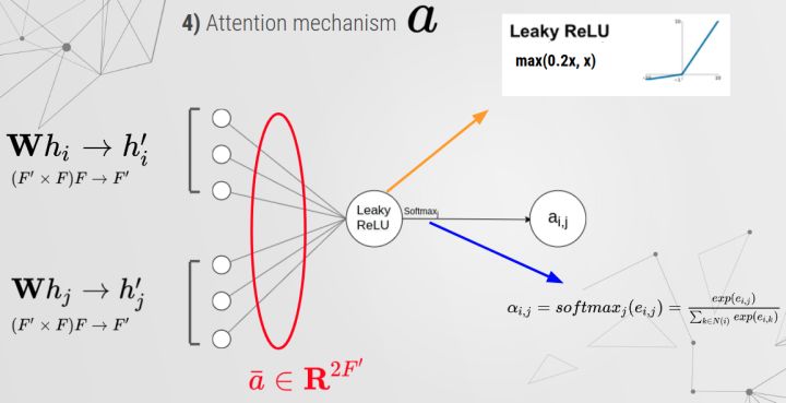
具体实现:

x = torch.tensor([[1, 2], [1, 3], [2, 3]])

a = nn.Parameter(torch.zeros(size=(2*out_features, 1)))
nn.init.xavier_uniform_(a.data, gain=1.414)
print(a.shape)

leakyrelu = nn.LeakyReLU(0.2)

# h = (3, 2), N = (3, )
# 1. W h_i = h_i' = ()
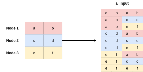
# 1. repeat N times of h => (3, 2 * 3)
# 2. change shape to (9, 2)
# 3. concat with another repeat N times of h => (9, 2), => (9, 4)
a_input = torch.cat([h.repeat(1, N).view(N * N, -1), h.repeat(N, 1)], dim=1)
a_input = a_input.view(N, -1, 2 * out_features)
print(a_input.shape)

输出结果:

torch.Size([4, 1])
torch.Size([3, 3, 4])

可视化这一过程如下:

Attention Mechanism

print(a_input.shape, a.shape)
print("")
print(torch.matmul(a_input,a).shape)
print("")
print(torch.matmul(a_input,a).squeeze(2).shape)

输出结果:

torch.Size([3, 3, 4]) torch.Size([4, 1])

torch.Size([3, 3, 1])

torch.Size([3, 3])

最后计算 $e_{i, j}$:

e = leakyrelu(torch.matmul(a_input, a).squeeze(2))

掩码注意力 (Masked Attention)

有时候我们并不需要所有的注意力, 比如有些节点之间不存在连接, 则这时候就需要使用掩码来去除对应的注意力, 使得一些值变成0 (或 “无限” 接近于0).

adj = torch.randint(2, (3, 3))
print("adjacency matrix:\n", adj)
print("e:\n", e)

zero_vec = -9e15 * torch.ones_like(e)
print("\nmask:\n", zero_vec)

attention = torch.where(adj > 0, e, zero_vec)
print("\nattention:\n", attention)

输出结果:

adjacency matrix:
 tensor([[1, 1, 0],
        [1, 1, 0],
        [0, 1, 0]])
e:
 tensor([[ 0.0321, -0.0440, -0.0709],
        [ 0.3137,  0.0614, -0.0146],
        [ 0.4647,  0.2123,  0.0781]], grad_fn=<LeakyReluBackward0>)

mask:
 tensor([[-9.0000e+15, -9.0000e+15, -9.0000e+15],
        [-9.0000e+15, -9.0000e+15, -9.0000e+15],
        [-9.0000e+15, -9.0000e+15, -9.0000e+15]])

attention:
 tensor([[ 3.2143e-02, -4.4035e-02, -9.0000e+15],
        [ 3.1371e-01,  6.1393e-02, -9.0000e+15],
        [-9.0000e+15,  2.1234e-01, -9.0000e+15]], grad_fn=<SWhereBackward0>)

注意, 因为我们之后会应用 softmax 函数, 所以我们使用 -9.0000e+15 而不是0.

对比输入和输出:

attention = F.softmax(attention, dim=1)
print("attention after softmax:\n", attention)

h_prime = torch.matmul(attention, h)
print('\ninput:\n', h)
print("\noutput with masked attention:\n", h_prime)

输出结果:

attention after softmax:
 tensor([[0.5190, 0.4810, 0.0000],
        [0.5627, 0.4373, 0.0000],
        [0.0000, 1.0000, 0.0000]], grad_fn=<SoftmaxBackward0>)

input:
 tensor([[ 0.6022, -0.2289],
        [ 0.1860, -0.0468],
        [ 0.4765, -0.1651]], grad_fn=<MmBackward0>)

output with masked attention:
 tensor([[ 0.4020, -0.1413],
        [ 0.4202, -0.1492],
        [ 0.1860, -0.0468]], grad_fn=<MmBackward0>)

构建 GAT 层

class GATLayer(nn.Module):
    def __init__(self, in_features, out_features, dropout, alpha, concat=True):
        super(GATLayer).__init__()
        self.in_features = in_features
        self.out_features = out_features
        self.dropout = dropout              # dropout probability = 0.6
        self.alpha = alpha                  # LeakyReLU with negative input slope, alpha = 0.2
        self.concat = concat                # concat is True for all layers except the output layer

        # Learnable parameters weight and attention
        # Xavier Initialization, alternatively use weights_init to apply weights of choice 
        self.W = torch.zeros((in_features, out_features))
        nn.init.xavier_uniform_(self.W.data, gain=1.414)
        self.a = nn.Parameter(torch.zeros(size=(2*out_features, 1)))
        nn.init.xavier_uniform_(self.a.data, gain=1.414)

        self.leakyrelu = nn.LeakyReLU(self.alpha)

    def forward(self, input, adj):
        # Linear Transformation
        h = torch.mm(input, self.W)
        N = h.size()[0]
        print(N)

        # Attention Mechanism
        a_input = torch.cat([h.repeat(1, N).view(N * N, -1), h.repeat(N, 1)], dim=1)
        e = self.leakyrelu(torch.matmul(a_input, self.a).squeeze(2))

        # Masked Attention
        zero_vec = -9e15 * torch.ones_like(e)
        attention = torch.where(adj > 0, e, zero_vec)

        attention = F.softmax(attention, dim=1)
        attention = F.dropout(attention, self.dropout, training=self.training)
        h_prime = torch.matmul(attention, h)

        if self.concat:
            return F.elu(h_prime)
        else:
            return h_prime

接下来让我们使用 PyG 提供的 GATConv 来处理节点分类任务.

训练GAT模型

from torch_geometric.data import Data
from torch_geometric.nn import GATConv
from torch_geometric.datasets import Planetoid
import torch_geometric.transforms as T

import matplotlib.pyplot as plt

name_data = 'Cora'
dataset = Planetoid(root = '/tmp/' + name_data, name=name_data)
dataset.transform = T.NormalizeFeatures()

print(f'Number of graphs: {len(dataset)}')
print(f"Number of Classes in {name_data}:", dataset.num_classes)
print(f"Number of Node Features in {name_data}:", dataset.num_node_features)

完整网络:

class GAT(torch.nn.Module):
    def __init__(self):
        super(GAT, self).__init__()
        self.hid = 8
        self.in_head = 8
        self.out_head = 1

        self.conv1 = GATConv(in_channels=dataset.num_features, 
                             out_channels=self.hid, 
                             heads=self.in_head, 
                             dropout=0.6)
        self.conv2 = GATConv(in_channels=self.hid * self.in_head, 
                             out_channels=dataset.num_classes, 
                             concat=False,
                             heads=self.out_head, 
                             dropout=0.6)
        
    def forward(self, data):
        x, edge_index = data.x, data.edge_index

        x = F.dropout(x, p=0.6, training=self.training)
        x = self.conv1(x, edge_index)
        x = F.elu(x)
        x = F.dropout(x, p=0.6, training=self.training)
        x = self.conv2(x, edge_index)

        return F.log_softmax(x, dim=1)

device = torch.device('cuda' if torch.cuda.is_available() else 'cpu')
device = "cpu"

model = GAT().to(device)
data = dataset[0].to(device)
optimizer = torch.optim.Adam(model.parameters(), lr=0.005, weight_decay=5e-4)

model.train()
for epoch in range(1000):
    model.train()
    optimizer.zero_grad()
    out = model(data)
    loss = F.nll_loss(out[data.train_mask], data.y[data.train_mask])

    if epoch % 200 == 0:
        print(loss)

    loss.backward()
    optimizer.step()

输出结果:

tensor(1.9421, grad_fn=<NllLossBackward0>)
tensor(0.5664, grad_fn=<NllLossBackward0>)
tensor(0.6280, grad_fn=<NllLossBackward0>)
tensor(0.5148, grad_fn=<NllLossBackward0>)
tensor(0.5664, grad_fn=<NllLossBackward0>)

评估模型性能

model.eval()
_, pred = model(data).max(dim=1)
correct = float(pred[data.test_mask].eq(data.y[data.test_mask]).sum().item())
acc = correct / data.test_mask.sum().item()
print('Accuracy: {:.4f}'.format(acc))

输出结果:

Accuracy: 0.8160

参考

原博文链接: https://pytorch-geometric.readthedocs.io/en/latest/notes/colabs.html

[1] Veličković, Petar, et al. “Graph attention networks.” arXiv preprint arXiv:1710.10903 (2017).

PREVIOUS学习资源

NEXTUC Berkeley CS285 深度强化学习的中文译本