下载并引入库
# Install required packages.
!pip install -q torch-scatter -f https://data.pyg.org/whl/torch-1.10.0+cu113.html
!pip install -q torch-sparse -f https://data.pyg.org/whl/torch-1.10.0+cu113.html
!pip install -q git+https://github.com/pyg-team/pytorch_geometric.git

# Helper function for visualization.
%matplotlib inline
import matplotlib.pyplot as plt
from sklearn.manifold import TSNE

def visualize(h, color):
    z = TSNE(n_components=2).fit_transform(h.detach().cpu().numpy())

    plt.figure(figsize=(10,10))
    plt.xticks([])
    plt.yticks([])

    plt.scatter(z[:, 0], z[:, 1], s=70, c=color, cmap="Set2")
    plt.show()
使用 GNN 进行节点分类 (Node Classification)
在这个教程中, 我们将涉及如何应用GNN到节点分类的任务中. 假设我们只知道节点的一个小子集的真实 (ground-truth) 标签, 并且想要推断所有剩余节点的标签 (直推学习 transductive learning).
为方便展示, 我们使用 Cora 数据集, 这是一个 引文网络 (citation network), 其中节点代表的是具体的文档. 我们用一个1433维的 词袋 (bag-of-words) 特征向量来描述每个节点. 如果两文档间存在一引用连接, 则我们认为在图中这两个节点是相连的. 我们的任务是推断每个文档的类别 (我们有7个类).
这个数据集第一次被 Yang et al. 引入, 作为 Planetoid 基准标件 (benchmark suite) 的数据集之一. 更多信息请参考 PyG 数据集.
from torch_geometric.datasets import Planetoid
from torch_geometric.transforms import NormalizeFeatures

dataset = Planetoid(root='data/Planetoid', name='Cora', transform=NormalizeFeatures())

print()
print(f'Dataset: {dataset}:')
print('======================')
print(f'Number of graphs: {len(dataset)}')
print(f'Number of features: {dataset.num_features}')
print(f'Number of classes: {dataset.num_classes}')

data = dataset[0]  # 获取第一个图对象

print()
print(data)
print('===========================================================================================================')

# Gather some statistics about the graph.
print(f'Number of nodes: {data.num_nodes}')
print(f'Number of edges: {data.num_edges}')
print(f'Average node degree: {data.num_edges / data.num_nodes:.2f}')
print(f'Number of training nodes: {data.train_mask.sum()}')
print(f'Training node label rate: {int(data.train_mask.sum()) / data.num_nodes:.2f}')
print(f'Has isolated nodes: {data.has_isolated_nodes()}')
print(f'Has self-loops: {data.has_self_loops()}')
print(f'Is undirected: {data.is_undirected()}')
输出结果:
Downloading https://github.com/kimiyoung/planetoid/raw/master/data/ind.cora.x
Downloading https://github.com/kimiyoung/planetoid/raw/master/data/ind.cora.tx
Downloading https://github.com/kimiyoung/planetoid/raw/master/data/ind.cora.allx
Downloading https://github.com/kimiyoung/planetoid/raw/master/data/ind.cora.y
Downloading https://github.com/kimiyoung/planetoid/raw/master/data/ind.cora.ty
Downloading https://github.com/kimiyoung/planetoid/raw/master/data/ind.cora.ally
Downloading https://github.com/kimiyoung/planetoid/raw/master/data/ind.cora.graph
Downloading https://github.com/kimiyoung/planetoid/raw/master/data/ind.cora.test.index
Processing...
Done!

Dataset: Cora():
======================
Number of graphs: 1
Number of features: 1433
Number of classes: 7

Data(x=[2708, 1433], edge_index=[2, 10556], y=[2708], train_mask=[2708], val_mask=[2708], test_mask=[2708])
===========================================================================================================
Number of nodes: 2708
Number of edges: 10556
Average node degree: 3.90
Number of training nodes: 140
Training node label rate: 0.05
Has isolated nodes: False
Has self-loops: False
Is undirected: True
整体来说, 这个数据集和之前用的 KarateClub 网络非常相似. 我们可以看到 Cora 网络拥有2708个节点和10556条边, 这导致了平均节点 出入度数 (in-degree/out-degree) 为 3.9 (10556/2708 = 3.898). 这里有个概念, 什么是出度和入度呢? 对于一个有向图来说, 某个节点的 出度 指的是有多少条边从该节点出发与其他节点相连, 而 入度 则是从其他节点出发, 有多少条边进入该节点. 需要注意的是, 对于一个无向图来说, 出度即为入度.
为了训练这个数据集, 我们已知的真实类别的节点有140个, 也就是每个类别各20个. 这意味着训练节点的标签率只有5%. 与 KarateClub 不同, 这次的图拥有额外的属性 val_mask 和 test_mask, 代表用来验证和测试的节点. 另外, 我们会通过函数功能transform=NormalizeFeatures() 来完成 数据变换 (data transformations). 在把数据输入至神经网络之前, 我们可以用使用转换来修改输入数据, 用于例如标准化或数据增强. 在这个教程中, 我们使用 行归一 (row-normalize) 的操作来归一化输入的词袋特征向量.
待会我们可以看到这个网络是无向的, 并且没有孤立节点, 也就是每篇文档至少有一个引用.
训练 多层感知机网络 (Multi-layer Perception Network, MLP)
理论上来说, 我们 仅会 基于一篇文档的内容, 也就是词袋特征表达, 就应该能够推断出它的类别, 而不需要考虑任何相关信息. 让我们通过构建一个简单的 MLP 来验证这一点. 该 MLP 进在输入节点特征上操作 (使用在所有节点上共享的权重):
import torch
from torch.nn import Linear
import torch.nn.functional as F


class MLP(torch.nn.Module):
    def __init__(self, hidden_channels):
        super().__init__()
        torch.manual_seed(12345)
        self.lin1 = Linear(dataset.num_features, hidden_channels)
        self.lin2 = Linear(hidden_channels, dataset.num_classes)

    def forward(self, x):
        x = self.lin1(x)
        x = x.relu()
        x = F.dropout(x, p=0.5, training=self.training)
        x = self.lin2(x)
        return x

model = MLP(hidden_channels=16)
print(model)
输出结果:
MLP(
  (lin1): Linear(in_features=1433, out_features=16, bias=True)
  (lin2): Linear(in_features=16, out_features=7, bias=True)
)
可以看出, MLP 有两线性层和增强用的非线性函数ReLU和dropout. 首先我们需要降维1433维的特征向量到一个低维的嵌入 hidden_channels=16, 而第二线性层的作用是归类, 它映射每个低纬度的节点嵌入到7个类别中的一个.
model = MLP(hidden_channels=16)
criterion = torch.nn.CrossEntropyLoss()  # Define loss criterion.
optimizer = torch.optim.Adam(model.parameters(), lr=0.01, weight_decay=5e-4)  # Define optimizer.

def train():
      model.train()
      optimizer.zero_grad()         # 清零梯度.
      out = model(data.x)           # 单次前向传播.
      # 基于训练节点单独计算损失.
      loss = criterion(out[data.train_mask], data.y[data.train_mask])
      loss.backward()   # 根据后向传播推导梯度.
      optimizer.step()  # 基于梯度更新参数.
      return loss

def test():
      model.eval()
      out = model(data.x)
      pred = out.argmax(dim=1)  # Use the class with highest probability.
      test_correct = pred[data.test_mask] == data.y[data.test_mask]  # Check against ground-truth labels.
      test_acc = int(test_correct.sum()) / int(data.test_mask.sum())  # Derive ratio of correct predictions.
      return test_acc

for epoch in range(1, 201):
    loss = train()
    print(f'Epoch: {epoch:03d}, Loss: {loss:.4f}')
输出结果:
Epoch: 001, Loss: 1.9615
...
Epoch: 050, Loss: 1.0563
...
Epoch: 100, Loss: 0.5350
...
Epoch: 150, Loss: 0.4212
...
Epoch: 200, Loss: 0.3810
在训练这个模型之后, 我们可以调用 test 函数来查看我们模型的性能如何. 我们关注模型的准确率, 也就是, 正确归类的节点的比例:
test_acc = test()
print(f'Test Accuracy: {test_acc:.4f}')
输出结果:
Test Accuracy: 0.5900
不难发现, MLP 的表现不怎么样, 仅有 59% 的测试准确率. 但是这是因为什么呢? 主要的原因是过拟合, 因为MLP只能获取很少部分的训练节点, 因此对于没见过的节点表达的泛化能力就降低了.
训练 GNN
要转换 MLP 到 GNN 很简答, 我们只需要改变 torch.nn.Linear 层为 PyG 的 GNN 操作器. 与前一个教程相同, 我们仍然使用 GCNConv 模块, 详情请参考 前一篇教程. 与 GCNConv 不同, 单一`Linear 层是这么定义的:
并不会用到邻近节点的信息.
from torch_geometric.nn import GCNConv


class GCN(torch.nn.Module):
    def __init__(self, hidden_channels):
        super().__init__()
        torch.manual_seed(1234567)
        self.conv1 = GCNConv(dataset.num_features, hidden_channels)
        self.conv2 = GCNConv(hidden_channels, dataset.num_classes)

    def forward(self, x, edge_index):
        x = self.conv1(x, edge_index)
        x = x.relu()
        x = F.dropout(x, p=0.5, training=self.training)
        x = self.conv2(x, edge_index)
        return x

model = GCN(hidden_channels=16)
print(model)
输出结果:
GCN(
  (conv1): GCNConv(1433, 16)
  (conv2): GCNConv(16, 7)
)
如果我们可视化未训练的GCN网络的节点嵌入. 注意在 visualize(h, color) 函数中, 因为我们的节点嵌入是7维的, 所以我们使用 t-SNE 在2D平面进行可视化:
model = GCN(hidden_channels=16)
model.eval()

out = model(data.x, data.edge_index)
visualize(out, color=data.y)
输出结果:
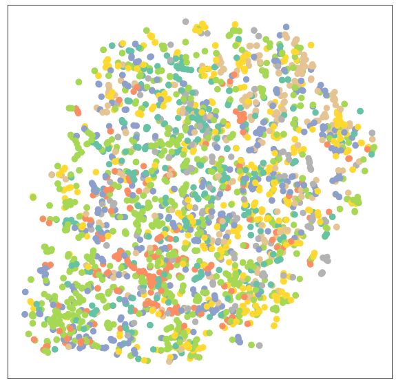
可以确信, 通过训练我们的模型, 它可以有更好的性能. 这次我们使用 节点特征 x 和 图连通性向量 edge_index 作为模型输入:
model = GCN(hidden_channels=16)
optimizer = torch.optim.Adam(model.parameters(), lr=0.01, weight_decay=5e-4)
criterion = torch.nn.CrossEntropyLoss()

def train():
      model.train()
      optimizer.zero_grad()  # Clear gradients.
      out = model(data.x, data.edge_index)  # Perform a single forward pass.
      # Compute the loss solely based on the training nodes.
      loss = criterion(out[data.train_mask], data.y[data.train_mask])
      loss.backward()   # Derive gradients.
      optimizer.step()  # Update parameters based on gradients.
      return loss

def test():
      model.eval()
      out = model(data.x, data.edge_index)
      pred = out.argmax(dim=1)  # Use the class with highest probability.
      test_correct = pred[data.test_mask] == data.y[data.test_mask]  # Check against ground-truth labels.
      test_acc = int(test_correct.sum()) / int(data.test_mask.sum())  # Derive ratio of correct predictions.
      return test_acc


for epoch in range(1, 101):
    loss = train()
    print(f'Epoch: {epoch:03d}, Loss: {loss:.4f}')
输出结果:
Epoch: 001, Loss: 1.9463
...
Epoch: 050, Loss: 1.1296
...
Epoch: 100, Loss: 0.5799
检查测试准确度:
test_acc = test()
print(f'Test Accuracy: {test_acc:.4f}')
输出结果:
Test Accuracy: 0.8150
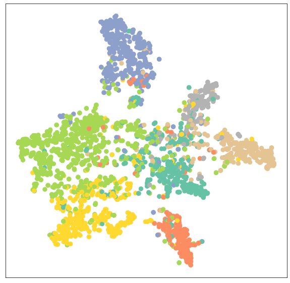
好耶! 通过简单地交换线性层为 GNN 层, 我们就能达到81.5%的测试准确度! 这与 MLP 59% 测试准确度形成了鲜明对比, 说明相关信息对获得更好的性能起着至关重要的作用. 我们也可以再次验证这一结果, 通过观察训练后模型的输出嵌入. 我们会发现这个模型现在可以对相同类别的节点进行更好地聚类 (cluster) 了.
model.eval()

out = model(data.x, data.edge_index)
visualize(out, color=data.y)
输出结果:
练习
- 为了获得更好的模型性能, 我们通常基于一个额外的验证集来选择最好的模型.
Cora数据集同样提供一个验证节点集合data.val_mask, 但是我们还没有用过. 你能修改上面的代码, 使得测试准确度的函数可以选择要测试的集合, 并且测试模型, 挑选出最高验证性能的模型吗? 最佳性能应该是82%准确率. - 当隐藏层特征维度增加, 或者层数增加, GCN 会有什么样的表现呢? 增加层数会有帮助吗?
- 我们可以尝试其他的GNN层来观察模型性能的改变. 比如我们使用
GATConv层 (包含多头注意力 multi-head attention), 尝试写出一个两层的GAT模型, 其在 第一层使用8头注意力, 在 第二层使用单头注意力, 并且在每次 内部调用时和外部调用后 都设置dropout比例为0.6, 并且每个头的hidden_channels都是8.
参考
原博文链接: https://pytorch-geometric.readthedocs.io/en/latest/notes/colabs.html