PyTorch Geometric 教程4 - 拓展图神经网络

下载库

# Install required packages.
!pip install -q torch-scatter -f https://data.pyg.org/whl/torch-1.10.0+cu113.html
!pip install -q torch-sparse -f https://data.pyg.org/whl/torch-1.10.0+cu113.html
!pip install -q git+https://github.com/pyg-team/pytorch_geometric.git

拓展 (Scaling) GNNs

之前的教程中, 我们仅以全批量 (full-batch) 的方式训练了节点分类任务中的 GNN. 这意味着每个节点的隐藏表达 (hidden representation) 都被并行地计算了, 在下一层, 我们依然可以重复使用. 但是, 一旦我们想要操作更大的图, 这一架构就不再行得通了, 因为内存消耗会 “爆炸”. 例如, 一个有着约1千万节点和128维隐藏特征的图需要每层消耗 5GB的 GPU 内存. 因此, 最近有不少科研人员致力于让 GNN 拓展到更大的规模. 有一种方法叫做 Cluster-GCN [1], 基于将图预先划分 (pre-partition) 成可以用小批量形式操作的子图. 接下来, 我们将从 Planetoid 加载 PubMed 图:

import torch
from torch_geometric.datasets import Planetoid
from torch_geometric.transforms import NormalizeFeatures

dataset = Planetoid(root='data/Planetoid', name='PubMed', transform=NormalizeFeatures())

print()
print(f'Dataset: {dataset}:')
print('==================')
print(f'Number of graphs: {len(dataset)}')
print(f'Number of features: {dataset.num_features}')
print(f'Number of classes: {dataset.num_classes}')

data = dataset[0]  # Get the first graph object.

print()
print(data)
print('===============================================================================================================')

# Gather some statistics about the graph.
print(f'Number of nodes: {data.num_nodes}')
print(f'Number of edges: {data.num_edges}')
print(f'Average node degree: {data.num_edges / data.num_nodes:.2f}')
print(f'Number of training nodes: {data.train_mask.sum()}')
print(f'Training node label rate: {int(data.train_mask.sum()) / data.num_nodes:.3f}')
print(f'Has isolated nodes: {data.has_isolated_nodes()}')
print(f'Has self-loops: {data.has_self_loops()}')
print(f'Is undirected: {data.is_undirected()}')

输出结果:

Dataset: PubMed():
==================
Number of graphs: 1
Number of features: 500
Number of classes: 3

Data(x=[19717, 500], edge_index=[2, 88648], y=[19717], train_mask=[19717], val_mask=[19717], test_mask=[19717])
===============================================================================================================
Number of nodes: 19717
Number of edges: 88648
Average node degree: 4.50
Number of training nodes: 60
Training node label rate: 0.003
Has isolated nodes: False
Has self-loops: False
Is undirected: True

不难发现, 这个图有19717个节点, 虽然这个数量的节点应该可以装入 GPU 的内存, 但这个数据集依然是个不错的例子, 它可以展示我们如何在 PyG 内拓展 GNNs.

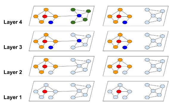
Cluster-GCN [1] 首先基于图划分算法 (graph partitioning algorithm) 来划分整图至多个子图. GNN 被限制为仅对其特定子图进行卷积操作, 从而避免了 领域爆炸 (neighborhood explosion) 的问题.

Graph partitioning

但是, 在图被划分之后, 一些连接被移除了, 这可能会因为有偏重 (biased) 的估计而限制模型的性能. 为了解决这一问题, Cluster-GCN 也在小批量中包含了集群 (cluster) 间的连接, 这也就是 随机划分架构 (stochastic partitioning scheme):

Stochastic graph partitioning

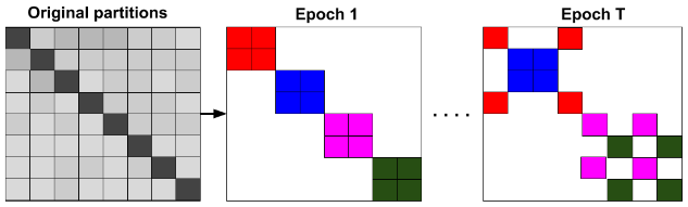
上图中, 颜色代表每个批量所维护的邻接信息, 需要注意的是, 每个 epoch 可能不同. PyG 提供 Cluster-GCN 算法的两步实现:

ClusterData 转换一个 Data 对象到子图的数据集, 这个数据集包含 num_parts 个划分
对于给定 batch_size, ClusterLoader 实施随机划分方案 (stochastic partioning scheme)

创造小批量的代码如下:

from torch_geometric.loader import ClusterData, ClusterLoader

torch.manual_seed(12345)
cluster_data = ClusterData(data, num_parts=128)  # 1. Create subgraphs.
train_loader = ClusterLoader(cluster_data, batch_size=32, shuffle=True)  # 2. Stochastic partioning scheme.

print()
total_num_nodes = 0
for step, sub_data in enumerate(train_loader):
    print(f'Step {step + 1}:')
    print('=======')
    print(f'Number of nodes in the current batch: {sub_data.num_nodes}')
    print(sub_data)
    print()
    total_num_nodes += sub_data.num_nodes

print(f'Iterated over {total_num_nodes} of {data.num_nodes} nodes!')

输出结果:

Computing METIS partitioning...

Step 1:
=======
Number of nodes in the current batch: 4928
Data(x=[4928, 500], y=[4928], train_mask=[4928], val_mask=[4928], test_mask=[4928], edge_index=[2, 16174])

Step 2:
=======
Number of nodes in the current batch: 4937
Data(x=[4937, 500], y=[4937], train_mask=[4937], val_mask=[4937], test_mask=[4937], edge_index=[2, 17832])

Step 3:
=======
Number of nodes in the current batch: 4927
Data(x=[4927, 500], y=[4927], train_mask=[4927], val_mask=[4927], test_mask=[4927], edge_index=[2, 14712])

Step 4:
=======
Number of nodes in the current batch: 4925
Data(x=[4925, 500], y=[4925], train_mask=[4925], val_mask=[4925], test_mask=[4925], edge_index=[2, 18006])

Iterated over 19717 of 19717 nodes!
Done!

在本例中, 我们划分初始图至128部分, 并且用有32张子图的 batch_size 来构建小批量 (这样每个 epoch 我们会有4个批量). 不难发现, 一个 epoch 之后, 每个节点只出现一次. Cluster-GCN 并不会让 GNN 模型变得更复杂, 我们仍然可以使用相同的结构:

import torch.nn.functional as F
from torch_geometric.nn import GCNConv

class GCN(torch.nn.Module):
    def __init__(self, hidden_channels):
        super(GCN, self).__init__()
        torch.manual_seed(12345)
        self.conv1 = GCNConv(dataset.num_node_features, hidden_channels)
        self.conv2 = GCNConv(hidden_channels, dataset.num_classes)

    def forward(self, x, edge_index):
        x = self.conv1(x, edge_index)
        x = x.relu()
        x = F.dropout(x, p=0.5, training=self.training)
        x = self.conv2(x, edge_index)
        return x

model = GCN(hidden_channels=16)
print(model)

输出结果:

GCN(
  (conv1): GCNConv(500, 16)
  (conv2): GCNConv(16, 3)
)

训练上面的 GNN 和训练图分类任务的 GNN 相似, 只不过后者是以全批量的方式操作图, 而我们现在需要在每个小批量进行迭代, 并单独优化每个批量:

model = GCN(hidden_channels=16)
optimizer = torch.optim.Adam(model.parameters(), lr=0.01, weight_decay=5e-4)
criterion = torch.nn.CrossEntropyLoss()

def train():
      model.train()

      for sub_data in train_loader:  # Iterate over each mini-batch.
          out = model(sub_data.x, sub_data.edge_index)  # Perform a single forward pass.
          # Compute the loss solely based on the training nodes.
          loss = criterion(out[sub_data.train_mask], sub_data.y[sub_data.train_mask])  
          loss.backward()  # Derive gradients.
          optimizer.step()  # Update parameters based on gradients.
          optimizer.zero_grad()  # Clear gradients.

def test():
      model.eval()
      out = model(data.x, data.edge_index)
      pred = out.argmax(dim=1)  # Use the class with highest probability.
      
      accs = []
      for mask in [data.train_mask, data.val_mask, data.test_mask]:
          correct = pred[mask] == data.y[mask]  # Check against ground-truth labels.
          accs.append(int(correct.sum()) / int(mask.sum()))  # Derive ratio of correct predictions.
      return accs

for epoch in range(1, 51):
    loss = train()
    train_acc, val_acc, test_acc = test()
    print(f'Epoch: {epoch:03d}, Train: {train_acc:.4f}, Val Acc: {val_acc:.4f}, Test Acc: {test_acc:.4f}')

输出结果:

Epoch: 001, Train: 0.3333, Val Acc: 0.4160, Test Acc: 0.4070
...
Epoch: 020, Train: 0.9667, Val Acc: 0.7820, Test Acc: 0.7710
...
Epoch: 040, Train: 0.9833, Val Acc: 0.8040, Test Acc: 0.7830
...
Epoch: 050, Train: 0.9833, Val Acc: 0.8000, Test Acc: 0.7970

参考

原博文链接: https://pytorch-geometric.readthedocs.io/en/latest/notes/colabs.html

[1] Chiang, Wei-Lin, et al. “Cluster-gcn: An efficient algorithm for training deep and large graph convolutional networks.” Proceedings of the 25th ACM SIGKDD International Conference on Knowledge Discovery & Data Mining. 2019.

PREVIOUSPyTorch Geometric 教程2 - 节点分类

NEXTPyTorch Geometric 教程3 - 图分类