下载库
# Install required packages.
!pip install -q torch-scatter -f https://data.pyg.org/whl/torch-1.10.0+cu113.html
!pip install -q torch-sparse -f https://data.pyg.org/whl/torch-1.10.0+cu113.html
!pip install -q git+https://github.com/pyg-team/pytorch_geometric.git
使用图神经网络来分类图
图分类 (Graph classification) 指的是对于已知的图数据集, 基于一些结构图的属性, 分类整张图的任务. 因此, 我们需要嵌入整张图, 并且使它们在某些任务下是线性可分的.
图分类中, 最常见的任务是 分子性质预测 (molecular property prediction), 其中一个分子被表达成一张图. 举个例子, 任务可以是推断一个分子是否抑制HIV病毒的复制. 多特蒙德工业大学收集了广泛的图分类数据集, 取名为 TUDatasets. 在 PyG 中, 我们可以通过 torch_geometric.datasets.TUDataset 来获取这个数据集. 让我们来加载 MUTAG 数据集:
import torch
from torch_geometric.datasets import TUDataset

dataset = TUDataset(root='data/TUDataset', name='MUTAG')

print()
print(f'Dataset: {dataset}:')
print('====================')
print(f'Number of graphs: {len(dataset)}')
print(f'Number of features: {dataset.num_features}')
print(f'Number of classes: {dataset.num_classes}')

data = dataset[0]  # Get the first graph object.

print()
print(data)
print('=============================================================')

# Gather some statistics about the first graph.
print(f'Number of nodes: {data.num_nodes}')
print(f'Number of edges: {data.num_edges}')
print(f'Average node degree: {data.num_edges / data.num_nodes:.2f}')
print(f'Has isolated nodes: {data.has_isolated_nodes()}')
print(f'Has self-loops: {data.has_self_loops()}')
print(f'Is undirected: {data.is_undirected()}')
输出结果:
Downloading https://www.chrsmrrs.com/graphkerneldatasets/MUTAG.zip
Extracting data/TUDataset/MUTAG/MUTAG.zip
Processing...

Dataset: MUTAG(188):
====================
Number of graphs: 188
Number of features: 7
Number of classes: 2

Data(edge_index=[2, 38], x=[17, 7], edge_attr=[38, 4], y=[1])
=============================================================
Number of nodes: 17
Number of edges: 38
Average node degree: 2.24
Has isolated nodes: False
Has self-loops: False
Is undirected: True
Done!
这个数据集提供 188张不同的图, 我们的任务是分类每张图到两个类别中的一个.
通过检查数据集的第一个图对象, 我们可以发现它有 17个节点 (每个节点有 7维的特征向量), 和 38条边 (平均节点出入度数 38/17=2.24), 每张图都有 一个图标签 y=[1]. 另外, 每条边还有额外的 4维边特征 (edge feature) edge_attr=[38, 4]. 但是, 为了让本教程足够简单, 我们不会使用这些额外特征.
PyG 提供一些便利函数来帮助我们更好地处理图数据集, 例如, 我们可以 洗牌 (shuffle) 数据集, 并使用前150个图作为训练集, 其余的用作测试:
torch.manual_seed(12345)
dataset = dataset.shuffle()

train_dataset = dataset[:150]
test_dataset = dataset[150:]

print(f'Number of training graphs: {len(train_dataset)}')
print(f'Number of test graphs: {len(test_dataset)}')
输出结果:
Number of training graphs: 150
Number of test graphs: 38
图的小批量 (mini-batching) 训练
既然在图分类数据集中的单张图都比较小, 我们可以在输入到 GNN 之前, 将这些图 “捆” 成多个批次进行训练, 这样可以保证充分 GPU 的利用率. 在图像或语言领域, 这一过程通常通过将每个样例 缩放 (rescaling) 或 填充 (padding) 为一组形状相等的数据来实现 (这样输入数据就多了一个额外的维度). 这个维度的长度等于在小批量中的样本个数, 我们通常称其为 batch_size.
但是, 对于 GNN 来说, 上述的两种方法都不可行, 或者说可能会导致不必要的内存消耗. 因此, PyG 使用另一种方法优化, 以取得高效的样本之间的并行. 在本例中, 多个 邻接矩阵 (adjacency matrix) 以对角阵的形式堆积, 也就是多个子图构建一个大图. 在节点维度里, 节点和其特征会 拼接 (concatenate) 在一起, 从而形成大图的节点信息:
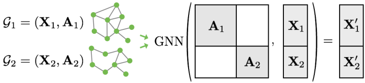
此程序与其他批处理程序相比有一些关键的优点:
- 依赖于信息传递架构的 GNN 操作器 (如 GCN 层) 不需要额外的修改. 这是因为不同图的节点之间不会进行消息交换.
- 没有计算或内存开销, 因为邻接矩阵是 稀疏的 (sparse), 也就是它只会保存非零的值, 也就是连通的边.
通过 torch_geometric.data.DataLoader 类, PyG 会自动地处理, 构建多个子图成一个批量的大图:
from torch_geometric.loader import DataLoader

train_loader = DataLoader(train_dataset, batch_size=64, shuffle=True)
test_loader = DataLoader(test_dataset, batch_size=64, shuffle=False)

for step, data in enumerate(train_loader):
    print(f'Step {step + 1}:')
    print('=======')
    print(f'Number of graphs in the current batch: {data.num_graphs}')
    print(data)
    print()
输出结果:
Step 1:
=======
Number of graphs in the current batch: 64
Batch(edge_attr=[2560, 4], edge_index=[2, 2560], x=[1154, 7], y=[64], batch=[1154], ptr=[65])

Step 2:
=======
Number of graphs in the current batch: 64
Batch(edge_attr=[2454, 4], edge_index=[2, 2454], x=[1121, 7], y=[64], batch=[1121], ptr=[65])

Step 3:
=======
Number of graphs in the current batch: 22
Batch(edge_attr=[980, 4], edge_index=[2, 980], x=[439, 7], y=[22], batch=[439], ptr=[23])
这里我们使用 batch_size=64, 这样我们会有3个小批量, 也就是包含 2 * 64 + 22 = 150 张图. 另外, 每个 Batch 对象都配有一个 赋值向量 (assignment vector) batch, 这个向量映射每个节点到它对应的批量里的图 $\text{batch} = [0, …, 0, 1, …, 1, 2, …]$.
训练 GNN
要训练 GNN 来进行图分类, 我们通常需要以下步骤:
- 通过执行多轮消息传递来嵌入每个节点
- 聚集 (aggregate) 节点嵌入 (node embedding) 到一个统一的 图嵌入 (graph embedding), 也就是读出层 (readout layer)
- 基于图嵌入来训练最终的分类器
文献中已有很多不同的 读出层, 但是最常用的只是简单地利用了节点嵌入的优势:
\[\mathbf{x_{G}} = \frac{1}{\| V \|} \sum_{v \in V} x_v^{(L)}\]PyG 也同样提供这一读出层 torch_geometric.nn.global_mean_pool, 该函数的输入为小批量内所有节点的节点嵌入和 赋值向量 (assignment vector) batch 来为批量内的每张图计算图嵌入 (形状为 [batch_size, hidden_channels]). 将 GNN 应用于图分类任务的最终架构如下所示:
from torch.nn import Linear
import torch.nn.functional as F
from torch_geometric.nn import GCNConv
from torch_geometric.nn import global_mean_pool


class GCN(torch.nn.Module):
    def __init__(self, hidden_channels):
        super(GCN, self).__init__()
        torch.manual_seed(12345)
        self.conv1 = GCNConv(dataset.num_node_features, hidden_channels)
        self.conv2 = GCNConv(hidden_channels, hidden_channels)
        self.conv3 = GCNConv(hidden_channels, hidden_channels)
        self.lin = Linear(hidden_channels, dataset.num_classes)

    def forward(self, x, edge_index, batch):
        # 1. Obtain node embeddings
        x = self.conv1(x, edge_index)
        x = x.relu()
        x = self.conv2(x, edge_index)
        x = x.relu()
        x = self.conv3(x, edge_index)

        # 2. Readout layer
        x = global_mean_pool(x, batch)  # [batch_size, hidden_channels]

        # 3. Apply a final classifier
        x = F.dropout(x, p=0.5, training=self.training)
        x = self.lin(x)

        return x

model = GCN(hidden_channels=64)
print(model)
输出结果:
GCN(
  (conv1): GCNConv(7, 64)
  (conv2): GCNConv(64, 64)
  (conv3): GCNConv(64, 64)
  (lin): Linear(in_features=64, out_features=2, bias=True)
)
在我们应用最后的分类器之前, 我们使用 GCNConv 和 $\text{ReLU}(x) = \max (x, 0)$ 激活函数, 来获得本地的节点嵌入, 现在让我们来训练这个网络:
model = GCN(hidden_channels=64)
optimizer = torch.optim.Adam(model.parameters(), lr=0.01)
criterion = torch.nn.CrossEntropyLoss()

def train():
    model.train()

    for data in train_loader:  # Iterate in batches over the training dataset.
        out = model(data.x, data.edge_index, data.batch)  # Perform a single forward pass.
        loss = criterion(out, data.y)  # Compute the loss.
        loss.backward()  # Derive gradients.
        optimizer.step()  # Update parameters based on gradients.
        optimizer.zero_grad()  # Clear gradients.

def test():
    model.eval()

    correct = 0
    for data in loader:  # Iterate in batches over the training/test dataset.
        out = model(data.x, data.edge_index, data.batch)
        pred = out.argmax(dim=1)  # Use the class with highest probability.
        correct += int((pred == data.y).sum())  # Check against ground-truth labels.
    return correct / len(loader.dataset)  # Derive ratio of correct predictions.

for epoch in range(1, 171):
    train()
    train_acc = test(train_loader)
    test_acc = test(test_loader)
    print(f'Epoch: {epoch:03d}, Train Acc: {train_acc:.4f}, Test Acc: {test_acc:.4f}')
输出结果:
Epoch: 001, Train Acc: 0.6467, Test Acc: 0.7368
...
Epoch: 050, Train Acc: 0.7667, Test Acc: 0.8158
...
Epoch: 100, Train Acc: 0.7733, Test Acc: 0.7895
...
Epoch: 150, Train Acc: 0.7800, Test Acc: 0.7895
...
Epoch: 170, Train Acc: 0.8000, Test Acc: 0.7632
不难发现, 我们的模型获得了大概 76%的测试准确度. 我们还可以观察到一些准确性波动, 这事因为我们的数据集比较小, 只有38个测试图, 一旦数据集增大, 这种波动通常就会消失.
练习
我们可以做得更好吗? 有不少的论文指出 [1, 2], 应用 领域归一化 (neighborhood normalization) 会降低 GNN 在区分某些图结构时的表达性. Morris 等提出的方法 [2] 完全避免了领域归一化, 并且为了保留中心节点的信息, 他们添加了一个简单的 残差连接 (skip-connection) 到 GNN 的层中:
\[\mathbf{x}_v^{(\ell+1)} = \mathbf{W}^{(\ell + 1)}_1 \mathbf{x}_v^{(\ell)} + \mathbf{W}^{(\ell + 1)}_2 \sum_{u \in \mathcal{N}(v)} \mathbf{x}_u^{(\ell)}\]在 PyG 中, 这一层叫做 GraphConv. 试试使用 GraphConv 来替换 GCNConv. 我们应该能得到接近 82% 的测试准确度.
参考
原博文链接: https://pytorch-geometric.readthedocs.io/en/latest/notes/colabs.html
[1] Xu, Keyulu, et al. “How powerful are graph neural networks?.” arXiv preprint arXiv:1810.00826 (2018).
[2] Morris, Christopher, et al. “Weisfeiler and leman go neural: Higher-order graph neural networks.” Proceedings of the AAAI conference on artificial intelligence. Vol. 33. No. 01. 2019.